Contents

Introduction

Kettlewell's Experiments

Table 1: Kettlewell's release-and-recapture data

Figure 1: The number of moths Kettlewell recaptured as a function of the number he released the previous night.

Figure 2: Kettlewell's recapture rate as a function of time.

Mathematical Model

Figure 3: A mathematical model fitted to Kettlewell's data.

Moonlight

Figure 4: Kettlewell's daily recapture rate as a function of relative exposure to moonlight.

Conclusion

References

Introduction

ernard Kettlewell did not cheat, or, more precisely, the evidence does not support the insinuation, widely repeated on the Internet, that he cheated.

Kettlewell was a distinguished naturalist whose studies on predation in peppered moths were a landmark in demonstrating natural selection in the wild. His studies are widely quoted and often used in textbook accounts of natural selection. Judith Hooper (2002), a journalist, strongly suggests, however, that Kettlewell fraudulently altered the results of his famous studies, and others  have uncritically accepted her suggestion.  Reviews of Hooper's book in the scientific literature are at best mixed (Coyne 2002, Grant 2002, Shapiro 2002), and experts on moth behavior remain convinced that the story of the peppered moth is sound (Cook, 2000, 2003; Grant 1999; Majerus 1998, 2003; Mallet 2004).   More pertinently, Kettlewell's data are completely consistent with normal experimental variation, and Hooper's insinuations are groundless.

Kettlewell's Experiments

What did Kettlewell do, and why does Hooper think he fudged his data?  Beginning in the mid-1800's, successive generations of peppered moths (Biston betularia) in Britain gradually darkened in response to the air pollution in the industrialized parts of the country.  Specifically, a genetically determined dark, or melanic, form of the moth replaced the lighter form as industrial pollution killed lichens on the barks of trees and also coated the bark with a layer of soot.  The effect has come to be known as industrial melanism, and its existence is not in dispute (see [Forrest and Gross, 2004: 107-111] for a review).

Kettlewell (1955, 1956, 1959) showed that the melanic form of the moth predominated primarily because of predation by birds. He did not think that predation was the only cause of industrial melanism and in fact speculated as to the relative strengths of other causes.  Briefly, he performed a number of experiments (Musgrave 2004, Grant 1999, Kettlewell 1959):

1. Release-recapture experiments.  Kettlewell marked and released both light-colored and melanic moths early in the morning, and recaptured some the next night.  In polluted woods, he and his assistants recaptured more melanic moths than light-colored (1955, 1956), whereas in unpolluted woods they captured more light-colored than melanic (1956).
2. Direct observation (1955, 1956) and filming (1956). Kettlewell and others observed birds eating moths directly off trunks of trees.
3. Camouflage.  Kettlewell visually ranked the effectiveness of camouflage of moths on different backgrounds and compared the effectiveness of camouflage with predation rates both in an aviary and in the field.  He did not know that birds had ultraviolet vision, which his observers lacked, but got nevertheless a good correlation between camouflage and predation.  Later research has shown that the moths are camouflaged in the ultraviolet as well as in the visible (Musgrave 2004).
4. Geographical distribution.  He noted that the distribution of the melanic moths in the country closely matched the areas of industrialization (Bishop and Cook 1957).

I  will discuss only the release-recapture experiments reported in (Kettlewell 1955), because these are the experiments that are under fire and because (unlike Kettlewell's critics) we can bring quantitative tools to bear.  For a more general analysis, see (Musgrave 2004; Grant 1999).

Kettlewell reported releasing and recapturing moths during an 11-day period in 1953.  His data are reproduced in Table 1 (1955: 332).  The numbering of the days is mine.

Hooper has noted that the number of recaptures increased sharply on 1 July, the same day that E. B. Ford sent a letter to Kettlewell.  Ford's letter commiserated with Kettlewell for the low recapture rates but suggested that the data would be worthwhile anyway.  The letter is unremarkable, and two facts militate against a finding of fraud. First, Kettlewell finished collecting data in the wee hours of the morning and therefore could not have received the letter before collecting his data on 1 July.  He  markedly increased the number of moths he released on 30 June, the day before the letter was mailed, not 1 July.  Additionally, as Hooper admits, he continued to release more moths after 30 June. Not surprisingly, he also captured more moths:  more moths released, more captured.

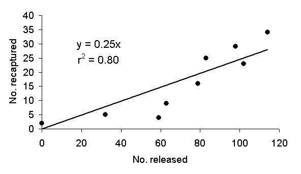Figure 1: The number of moths Kettlewell recaptured as a function of the number he released the previous night. The relationship is linear with a high correlation.

Indeed, Figure 1 plots recapture rate as a function of the number of moths released on any day.  The line is a line of best fit constrained to pass through the origin on the assumption that no moths are recaptured if none are released.  Figure 1 shows that the recapture rate is very nearly a linear function of the number released.  The square r² of the correlation coefficient is 0.80 and suggests that most of the variation of the number of recaptures is accounted for by variation of the number of releases.  The fit improves only slightly if the line is not constrained.

Why did Kettlewell release more moths beginning on 30 June?  He released both moths he had reared and moths he had captured.  Because the moths were just hatching, he had limited control of the number he could release on any given day.  There is no reason to suspect that the increased numbers of releases reflect anything other than the number of moths that were available.  At any rate, Ford's letter could not have influenced his decision to release more moths because it arrived after Kettlewell's first big release on 30 June.

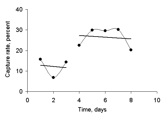Figure 2: Kettlewell's recapture rate as a function of time, ignoring the 2 days following 0 releases. Note that, owing to the vagaries of graphing programs, the days are not numbered correctly.

Still, his recapture rate, as well as the absolute number of moths recaptured, increased from 12 % over the first 3 days of his experiment to 26 % over the last 3 days.  More pointedly, if we plot his recapture rate as a function of time, as in Figure 2, we find what looks to the eye as a sudden increase.

Figure 2 omits those days, 27 June and 30 June, that were preceded by 0 releases.  It is hard to make much out of a mere 8 data points, but the recapture rate certainly appears to the casual observer to increase sharply after 1 day of inactivity. Biological field data, however, display significant random variation, and the eye often infers patterns in random data, so let us perform a quantitative analysis to see whether Kettlewell's data are what we would expect given normal experimental variations. Specifically, let us construct a mathematical model and see how well it describes Kettlewell's data.

Mathematical Model

Kettlewell recaptured most of his moths after they had been in the wild for only 1 day, but he recaptured some after 2 days. Let us therefore define a 1-day recapture rate R₁ and a 2-day recapture rate R₂ as the ratios of the numbers of moths recaptured after 1 and 2 days in the wild.  Kettlewell reported no 3-day recaptures.

We may estimate the 2-day recapture rate by looking at the 4 moths captured on days 2 and 5.  No moths were released on the preceding days, but 2 days before, a total of 63 -- 32 = 95 moths had been released, so R₂ = 4/95, or approximately 4 %.  The overall recapture rate is given by the row labeled "Totals" and is R = 149/630, or approximately 24 %.  The 1-day recapture rate is the difference R₁ = R - R₂ between the two values, or about 19 % (the numbers do not add exactly because of round-off error).  R₂ is very nearly equal to the square of R₁, as we would expect if the model is appropriate.

Our mathematical model is straightforward: The number of moths captured on any given night is equal to the number of moths released the day before times the 1-day recapture rate, plus a similar term, the number of moths released 2 days before times the 2-day recapture rate.  The results of a calculation based on this model are shown as the solid curve in Figure 3.  Note that I have made no artificial assumptions, such as adjusting the recapture rates to get a good fit to the data, in constructing Figure 3.

The points in Figure 3 are Kettlewell's data, and the solid curve is the model.  How well does the model fit the data?  To answer that question, we have to estimate the normal range of variability in the data.  In statistical terms, we calculate the standard uncertainty of the data points. The standard uncertainty is a number that tells us, in this case, how much variation we might expect if we repeated the experiment many times.

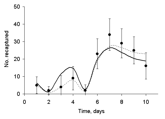Figure 3: A mathematical model fitted to Kettlewell's data. The points are the experimental data; the solid curve is the model, and the error bars are 95% confidence. The dashed curve is the model corrected for exposure to moonlight.

By way of introduction, suppose that you toss N marbles at a hole in a table.  Count the number of marbles that fall through the hole, and repeat the experiment many times.  Suppose that the average number of marbles that fall through the hole is M. You will not count M marbles every time you perform the experiment; to the contrary, the number will vary about M and very possibly will never exactly equal M. Thus, we talk of the probability p that any one marble passes through the hole and set it equal to the ratio M/N.  The mean number of marbles that pass through the hole is equal to Np.

How much will any one toss differ from M? Assume that the number of marbles that pass through the hole is described by a binomial distribution. Then the standard deviation of M is .  On approximately 19 tosses in 20, you will record a number that is between M - 2σ and M + 2σ, so 2σ is most commonly used as a measure of uncertainty.

The uncertainty 2σ can be surprisingly large.  For example, if p is 0.24 (the average recapture rate in Kettlewell's experiment) and N is 102 (the number of moths Kettlewell released on 30 June), then M is 24 and 2σ is about 8.  You can expect anywhere between 16 and 32 marbles to fall through the hole on any given toss.  You should not be especially surprised by any number unless it is much less than 12 or much more than 36. Thus, the day-to-day variation in an experiment such as Kettlewell's can easily be 100 % or more.  This fact alone should militate against a charge of fraud.

On any given day, Kettlewell released N moths and recaptured M moths.  Because the 2-day recapture rate is small, the statistics are essentially the same as those of the marble example.  The number M is highly variable, as we have seen; on another day, he might capture a substantially different number, even if conditions were unchanged.  The standard uncertainty u estimates the probable variation of M quantitatively (ISO 1993).  It is given by , where the recapture rate R replaces the probability p.  We apply this formula to each data point, using the overall recapture rate R for most days but the 2-day recapture rate R₂ for the 2 days that were preceded by 0 releases.

The result is shown in Figure 2 as a series of error bars.  The error bars represent ±2u, an interval called the 95 % confidence interval.  If we take a single measurement, then we may estimate that the true value (the average of a great many measurements) falls within the error bars, with 95 % probability. Inasmuch as the model (the solid curve) passes through virtually every error bar, it may be said to be a nearly perfect fit to the data, however poor it might appear in the absence of error bars.

The points on days 7, 8, and 9 lie noticeably above the curve.  If the data were completely unbiased, then we would expect about a 50-50 chance that any one of those points lay above the curve.  The odds that 3 consecutive points lie above the curve are 1 in 8, exactly the same as the odds against tossing 3 heads in a row and by no means improbable enough to base a charge of cheating.  Even if 5 points lay above the curve, the odds against would be 1 in 32, again, not very impressive in its improbability.  Additionally, 2 consecutive data points lie noticeably below the curve.

In summary, the last 5 of Kettlewell's data points are higher than the first 5.  This meager fact, combined with the anecdotal evidence of Ford's letter, is all that led Hooper (2003) to infer that Kettlewell cheated.  In reality, the timing of Ford's letter belies Hooper's inference, and Kettlewell's data are completely consistent with normal experimental variation.

Moonlight

The differences between the data and the curve are not statistically significant; the observed variation very probably is the result of chance.  It is, however, possible that the deviations from the curve are "real", that is, due to some systematic effect, or systematic error, not due solely to random error.  It is very hard, unfortunately, to track down a source of systematic error when that error is itself less than the standard uncertainty of the data set; the systematic error is said to be lost in the noise.

Hooper tells us that the weather was stable and could not have accounted for the increase in the number of recaptures (though her description suggests somewhat variable winds).  We have, nevertheless, a strong candidate that can account for the systematic deviations of our simple model from the curve: the phase of the moon. Shapiro (2002), in his review of Hooper's book, suggests that moonlight interferes with moth trapping, a possibility that Hooper and her informant, biologist Ted Sargent, should have investigated.  The moon was full on 27 June (that is, the night of 26-27 June).  By 2 July, the moon was 5 days past full but visible for only part of the night.  Thus, the total exposure to the moon, the product of illuminance (brightness) and time, was approximately one-quarter what it was during the full moon, and it dropped steadily over the next few days.

Clarke and his colleagues (1990) have investigated the effect of the phase of the moon on capture rates of peppered moths in a single environment over 30 years and concluded that the moon does not affect capture rates.  Unfortunately, theirs was a retrospective study, and they did not record weather data, that is, did not control for cloudy or rainy days.  They averaged the data over 5-day periods surrounding the full moon and did not use the actual exposure to the moonlight (as defined above). All of these factors will reduce the correlation between capture rates and exposure to moonlight.  Even so, they calculated a small but not statistically significant correlation that suggests a slight increase of capture rate around the full moon.  In addition, when they checked the new moon against the full moon, they calculated a small, barely significant increase, which they discounted.  Possibly the effect is due to the presence of streetlights, to which they refer obliquely, and which may attract moths away from the stronger mercury vapor light only when the moon is dark.  At any rate, they conclude that moonlight does not affect capture rates.  Kettlewell worked on clear days only; I do not think that the conclusion of Clarke and colleagues is necessarily pertinent.

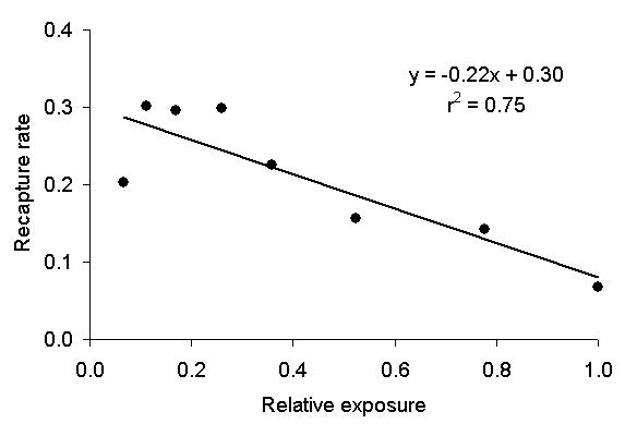Figure 4: Kettlewell's daily recapture rate as a function of relative exposure to moonlight. The equation is a line of best fit that relates exposure to recapture rate.

Thus, I examined Kettlewell's data in hope of quantifying the effect of the moon on his recapture rates (1955: 332, Table 5).  I obtained data that gave the moon's magnitude (an astronomical term that is related to its brightness) and the duration during which the moon was visible each night during Kettlewell's experiment. I plotted Kettlewell's daily recapture rate as a function of the exposure to the moon (the product of brightness and time, as defined above).  I made no effort to control for the elevation of the moon.  The result is shown in Figure 4, which plots Kettlewell's daily recapture rate as a function of lunar exposure normalized to the value 1 on the night of the full moon.  The equation in Figure 4 is the equation of the line of best fit to the data. The daily recapture rate rises by a factor of 3 as the brightness of the moon decreases.  (We could perform a similar calculation using Kettlewell's total captures  [1955: 333, Table 6], but such a calculation is complicated by the fact that the moths emerge from their cocoons haphazardly, whereas the recapture rate is based on a known distribution of released moths.  Still, the calculation based on total captures yields much the same result as that outlined below.)

Using the line in Figure 4, I adjusted the calculated recapture rates according to the equation,

where R represents the nightly recapture rate used in the model that led to Figure 3, R' is the nightly recapture rate modified to include the effect of lunar exposure, is the average daily recapture rate, and E is the nightly exposure to moonlight.  The result of the calculation is shown in Figure 3 as the light, dashed curve.  It demonstrates a somewhat better fit to the data than the solid curve, especially during the first few days.  Instead of asking why Kettlewell's recapture rate was high on 1 July and thereafter, Hooper should have asked why it was so low on 30 June and before.

Conclusion

Kettlewell's data are simply accounted for by the unsurprising fact that you can recapture more moths when you release more, that and normal experimental variation.  When the effect of moonlight is included in the calculation, the calculated curve fits even closer to Kettlewell's data.  We have no need of Hooper's perverse, ad-hoc hypothesis.

Hooper's claims are moonshine; they are based on a lack of understanding of Kettlewell's experiments in particular and experimental science in general.  Hooper evidently did not consider the most likely cause of the changes she saw, exposure to moonlight, let alone realize that the change in recapture numbers began before Kettlewell could have read the letter that supposedly triggered this change.  Hooper and Sargent should have performed a careful analysis before Hooper presumptuously insinuated fraud.

Kettlewell's conclusion, that predation by birds was a major factor in promoting industrial melanism, was based on at least 4 lines of inquiry, as detailed above.  It did not rely on the release-recapture experiments alone.  It is also supported by at least 30 studies of different moth species that also developed melanic forms (Grant, 1999).   In other words, an enormous body of evidence supports Kettlewell's conclusion.  Even if Kettlewell's release-recapture experiments were ruled out, we would still be forced to conclude that industrial melanism is the result of natural selection due to bird predation, possibly among other causes.

Thus, there is no foundation for assuming that Kettlewell's data were manipulated  The variations in his data are no more than the uncertainties associated with sampling and other factors, possibly including exposure to the moon. It is an irresponsible leap to accuse a distinguished naturalist of fraud on the basis of a single letter and a wholly imperfect, offhand analysis of his data.  The peppered moth properly remains a valid paradigm, no, an icon, of evolution.

Acknowledgements

Ian Musgrave provided the lunar data.  I am further indebted to Pete Dunkelberg and Bruce Grant for helping me understand the uncertainties of field work in biology.  Musgrave, Laurence Cook, and Nicholas Matzke reviewed the paper and made many helpful suggestions regarding both clarity and content.

Copyright © 2004 by Matt Young.  All rights reserved.  This paper may be reproduced on the Worldwide Web on condition that it be reproduced in its entirety and that the author be notified.  Print or hard-copy reproduction requires the express written consent of the author.

Matt Young is a former physicist with the US National Institute of Standards and Technology and now teaches physics and engineering at the Colorado School of Mines.  He is the author of No Sense of Obligation: Science and Religion in an Impersonal Universe (1st Books Library, 2001) and coeditor of Why Intelligent Design Fails: A Scientific Critique of the New Creationism (Rutgers University Press, 2004).

References

Clarke, Cyril A., Frieda  M. M. Clarke, H. C. Dawkins, and Susannah Kahtan (1990). "The Role of Moonlight in the Size of Catches of Biston betularia in West Kirby, Wirral, 1959-1988," Bulletin of the Amateur Entomologists' Society 368: 19-29.

Cook, L. M.  (2000). "Changing Views on Melanic Moths," Biological Journal of the Linnean Society 69: 431-441.

Cook, Laurence M. (2003).  "The Rise and Fall of the Carbonaria Form of the Peppered Moth," The Quarterly Review of Biology 78(4): 1-19.

Coyne, Jerry (2002).  "Evolution under Pressure," Nature 418: 20-21.

Grant, Bruce (1999).  "Fine Tuning the Peppered Moth," Evolution 53: 980-984.

Grant, Bruce (2002).  "Sour Grapes of Wrath," Science 297: 940-941.

Forrest, Barbara, and Paul R. Gross (2004).  Creationism's Trojan Horse: The Wedge of Intelligent Design.  New York: Oxford University Press.

Hooper, Judith (2002).  Of Moths and Men: An Evolutionary Tale.  New York: W.W. Norton.

ISO (1993).  Guide to the Expression of Uncertainty in Measurement. Geneva: International Organization for Standardization.

Kettlewell, H. B. D. (1955). "Selection Experiments on Industrial Melanism in the Lepidoptera," Heredity 9: 323-342.

Kettlewell, H. B. D. (1956). "Further Selection Experiments on Industrial Melanism in the Lepidoptera," Heredity 10 (Part 3): 287-301.

Majerus, M. E. N. (1998). Melanism: Evolution in Action. Oxford: Oxford University Press.  Chapter 6.

Majerus, M. E. N.  (2002). Moths.  London: HarperCollins.  Chapter 9.

Mallet, Jim (2002).  "The Peppered Moth: A Black and White Story after All," Genetical Society Newsletter, in press.  Available at http://abacus.gene.ucl.uk/jim/pap/malletgensoc03.pdf.

Musgrave, Ian (2004).  "Paint It Black: The Peppered Moth Story," in press.

Shapiro, Arthur M. (2002). "Paint It Black," Evolution 56: 1885-1886.